Step 4

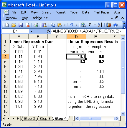
This screen shot shows a finished version of the spreadsheet. The 2x2 region D4:E5 has been formatted bold and it shows the four item we want returned. Cell D4 is selected and the function edit area shows the content of the cell. Note the braces "{..}" surrounding the "=LINEST(..)" that show you have correctly created an array function. Cells E7-E10 copy the data from the D4:E5 rectangle into a more readable format with individual labels.

The project is complete. A second task might be to select the data region A2:B14 (including its headers) and use the Chart Wizard to graph the data.

Back  Home